Following is the Logistic Regression analysis of the Challenger data.
## Example: Space Shuttle Launch Data ----
launch <- read.csv("C:/Users/Bhawna/Documents/blog/data/challenger.csv")

# examine the launch data
str(launch)
## 'data.frame': 23 obs. of 4 variables:
## $ distress_ct : int 0 1 0 0 0 0 0 0 1 1 ...
## $ temperature : int 66 70 69 68 67 72 73 70 57 63 ...
## $ field_check_pressure: int 50 50 50 50 50 50 100 100 200 200 ...
## $ flight_num : int 1 2 3 4 5 6 7 8 9 10 ...# logisitic regression
# First recode the distress_ct variable into 0 and 1, making 1 to represent at least
# one failure during a launch.
launch$distress_ct = ifelse(launch$distress_ct<1,0,1)
launch$distress_ct## [1] 0 1 0 0 0 0 0 0 1 1 1 0 0 1 0 0 0 0 0 0 1 0 1# set up trainning and test data sets
indx = sample(1:nrow(launch), as.integer(0.9*nrow(launch)))
indx## [1] 22 21 23 14 15 1 13 12 3 5 20 9 2 18 16 17 6 19 7 10launch_train = launch[indx,]
launch_test = launch[-indx,]
launch_train_labels = launch[indx,1]
launch_test_labels = launch[-indx,1] # Check if there are any missing values
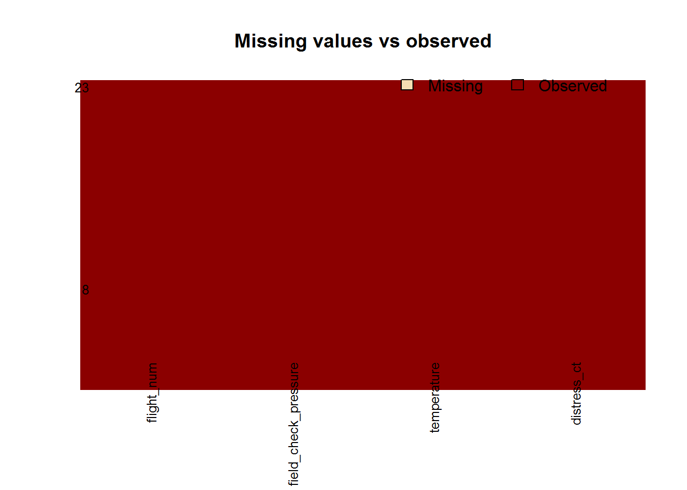
library(Amelia)## Warning: package 'Amelia' was built under R version 3.3.3## Loading required package: Rcpp## ##
## ## Amelia II: Multiple Imputation
## ## (Version 1.7.4, built: 2015-12-05)
## ## Copyright (C) 2005-2017 James Honaker, Gary King and Matthew Blackwell
## ## Refer to http://gking.harvard.edu/amelia/ for more information
## ##missmap(launch, main = "Missing values vs observed")
# number of missing values in each column

sapply(launch,function(x) sum(is.na(x)))
## distress_ct temperature field_check_pressure
## 0 0 0
## flight_num
## 0# number of unique values in each column
sapply(launch, function(x) length(unique(x)))## distress_ct temperature field_check_pressure
## 2 16 3
## flight_num
## 23# fit the logistic regression model, with all predictor variables
model <- glm(distress_ct ~.,family=binomial(link='logit'),data=launch_train)
model##
## Call: glm(formula = distress_ct ~ ., family = binomial(link = "logit"),
## data = launch_train)
##
## Coefficients:
## (Intercept) temperature field_check_pressure
## 17.108394 -0.273913 -0.003051
## flight_num
## 0.104614
##
## Degrees of Freedom: 19 Total (i.e. Null); 16 Residual
## Null Deviance: 24.43
## Residual Deviance: 15.46 AIC: 23.46summary(model)##
## Call:
## glm(formula = distress_ct ~ ., family = binomial(link = "logit"),
## data = launch_train)
##
## Deviance Residuals:
## Min 1Q Median 3Q Max
## -1.0591 -0.6450 -0.4137 0.2652 2.0663
##
## Coefficients:
## Estimate Std. Error z value Pr(>|z|)
## (Intercept) 17.108394 10.938385 1.564 0.1178
## temperature -0.273913 0.156348 -1.752 0.0798 .
## field_check_pressure -0.003051 0.021449 -0.142 0.8869
## flight_num 0.104614 0.240810 0.434 0.6640
## ---
## Signif. codes: 0 '***' 0.001 '**' 0.01 '*' 0.05 '.' 0.1 ' ' 1
##
## (Dispersion parameter for binomial family taken to be 1)
##
## Null deviance: 24.435 on 19 degrees of freedom
## Residual deviance: 15.456 on 16 degrees of freedom
## AIC: 23.456
##
## Number of Fisher Scoring iterations: 5anova(model, test="Chisq")## Analysis of Deviance Table
##
## Model: binomial, link: logit
##
## Response: distress_ct
##
## Terms added sequentially (first to last)
##
##
## Df Deviance Resid. Df Resid. Dev Pr(>Chi)
## NULL 19 24.435
## temperature 1 8.3938 18 16.041 0.003765 **
## field_check_pressure 1 0.3644 17 15.676 0.546073
## flight_num 1 0.2204 16 15.456 0.638722
## ---
## Signif. codes: 0 '***' 0.001 '**' 0.01 '*' 0.05 '.' 0.1 ' ' 1# drop the insignificant predictors, alpha = 0.10
model <- glm(distress_ct ~ temperature,family=binomial(link='logit'),data=launch_train)
model##
## Call: glm(formula = distress_ct ~ temperature, family = binomial(link = "logit"),
## data = launch_train)
##
## Coefficients:
## (Intercept) temperature
## 15.9552 -0.2469
##
## Degrees of Freedom: 19 Total (i.e. Null); 18 Residual
## Null Deviance: 24.43
## Residual Deviance: 16.04 AIC: 20.04summary(model)##
## Call:
## glm(formula = distress_ct ~ temperature, family = binomial(link = "logit"),
## data = launch_train)
##
## Deviance Residuals:
## Min 1Q Median 3Q Max
## -1.0370 -0.7056 -0.3422 0.3822 2.2961
##
## Coefficients:
## Estimate Std. Error z value Pr(>|z|)
## (Intercept) 15.9552 7.8268 2.039 0.0415 *
## temperature -0.2469 0.1156 -2.136 0.0327 *
## ---
## Signif. codes: 0 '***' 0.001 '**' 0.01 '*' 0.05 '.' 0.1 ' ' 1
##
## (Dispersion parameter for binomial family taken to be 1)
##
## Null deviance: 24.435 on 19 degrees of freedom
## Residual deviance: 16.041 on 18 degrees of freedom
## AIC: 20.041
##
## Number of Fisher Scoring iterations: 5anova(model, test="Chisq")## Analysis of Deviance Table
##
## Model: binomial, link: logit
##
## Response: distress_ct
##
## Terms added sequentially (first to last)
##
##
## Df Deviance Resid. Df Resid. Dev Pr(>Chi)
## NULL 19 24.435
## temperature 1 8.3938 18 16.041 0.003765 **
## ---
## Signif. codes: 0 '***' 0.001 '**' 0.01 '*' 0.05 '.' 0.1 ' ' 1# check Accuracy
fitted.results <- predict(model,newdata=launch_test,type='response')
fitted.results <- ifelse(fitted.results > 0.5,1,0)
misClasificError <- mean(fitted.results != launch_test$distress_ct)
print(paste('Accuracy',1-misClasificError))## [1] "Accuracy 0.666666666666667"# ROC
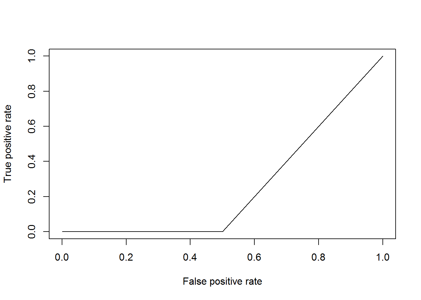
# Because this data set is so small, it is possible that the test data set
# does not contain both 0 and 1 values. If this happens the code will not
# run. And since the test data set is so small the ROC is not useful here
# but the code is provided.
library(ROCR)## Warning: package 'ROCR' was built under R version 3.3.3## Loading required package: gplots##
## Attaching package: 'gplots'## The following object is masked from 'package:stats':
##
## lowess## Loading required package: methodsp <- predict(model, newdata=launch_test, type="response")
pr <- prediction(p, launch_test$distress_ct)
prf <- performance(pr, measure = "tpr", x.measure = "fpr")
plot(prf)
auc <- performance(pr, measure = "auc")
auc <- auc@y.values[[1]]
Share this post
Twitter
Google+
Facebook
Reddit
LinkedIn
StumbleUpon
Email