Here we explore time series type dataset. Inbuilt Airpassenger dataset was used.
Load the data set notice Class is labeled “ts”-indicating a time series format
data("AirPassengers")
class(AirPassengers)
## [1] "ts"end(AirPassengers)## [1] 1960 12We can define the cycle of this time series in years
frequency(24)## [1] 1Summary
summary(AirPassengers)## Min. 1st Qu. Median Mean 3rd Qu. Max.
## 104.0 180.0 265.5 280.3 360.5 622.0plot(AirPassengers)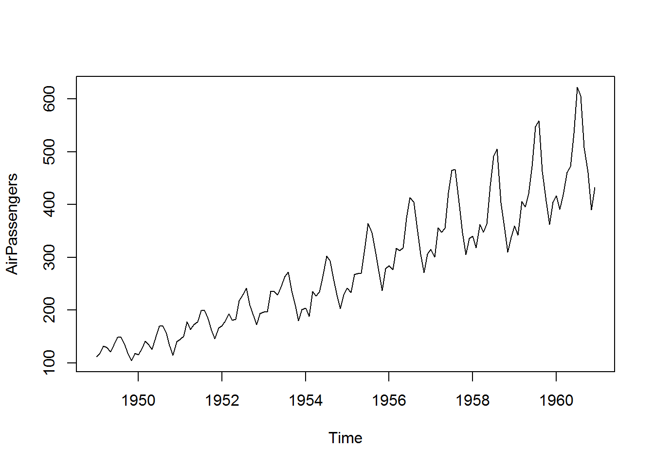
plot(AirPassengers)
abline(reg= lm (AirPassengers~time(AirPassengers)))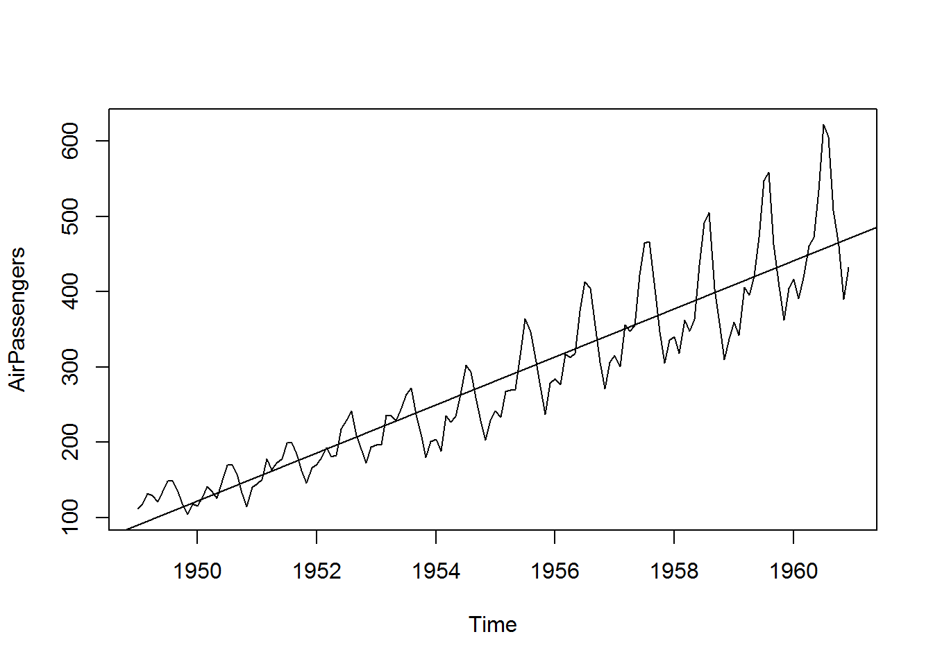
## pritn cycle across years, then aggregate cycles and display a year on year trend
cycle(AirPassengers)
## Jan Feb Mar Apr May Jun Jul Aug Sep Oct Nov Dec
## 1949 1 2 3 4 5 6 7 8 9 10 11 12
## 1950 1 2 3 4 5 6 7 8 9 10 11 12
## 1951 1 2 3 4 5 6 7 8 9 10 11 12
## 1952 1 2 3 4 5 6 7 8 9 10 11 12
## 1953 1 2 3 4 5 6 7 8 9 10 11 12
## 1954 1 2 3 4 5 6 7 8 9 10 11 12
## 1955 1 2 3 4 5 6 7 8 9 10 11 12
## 1956 1 2 3 4 5 6 7 8 9 10 11 12
## 1957 1 2 3 4 5 6 7 8 9 10 11 12
## 1958 1 2 3 4 5 6 7 8 9 10 11 12
## 1959 1 2 3 4 5 6 7 8 9 10 11 12
## 1960 1 2 3 4 5 6 7 8 9 10 11 12plot(aggregate(AirPassengers,FUN = mean))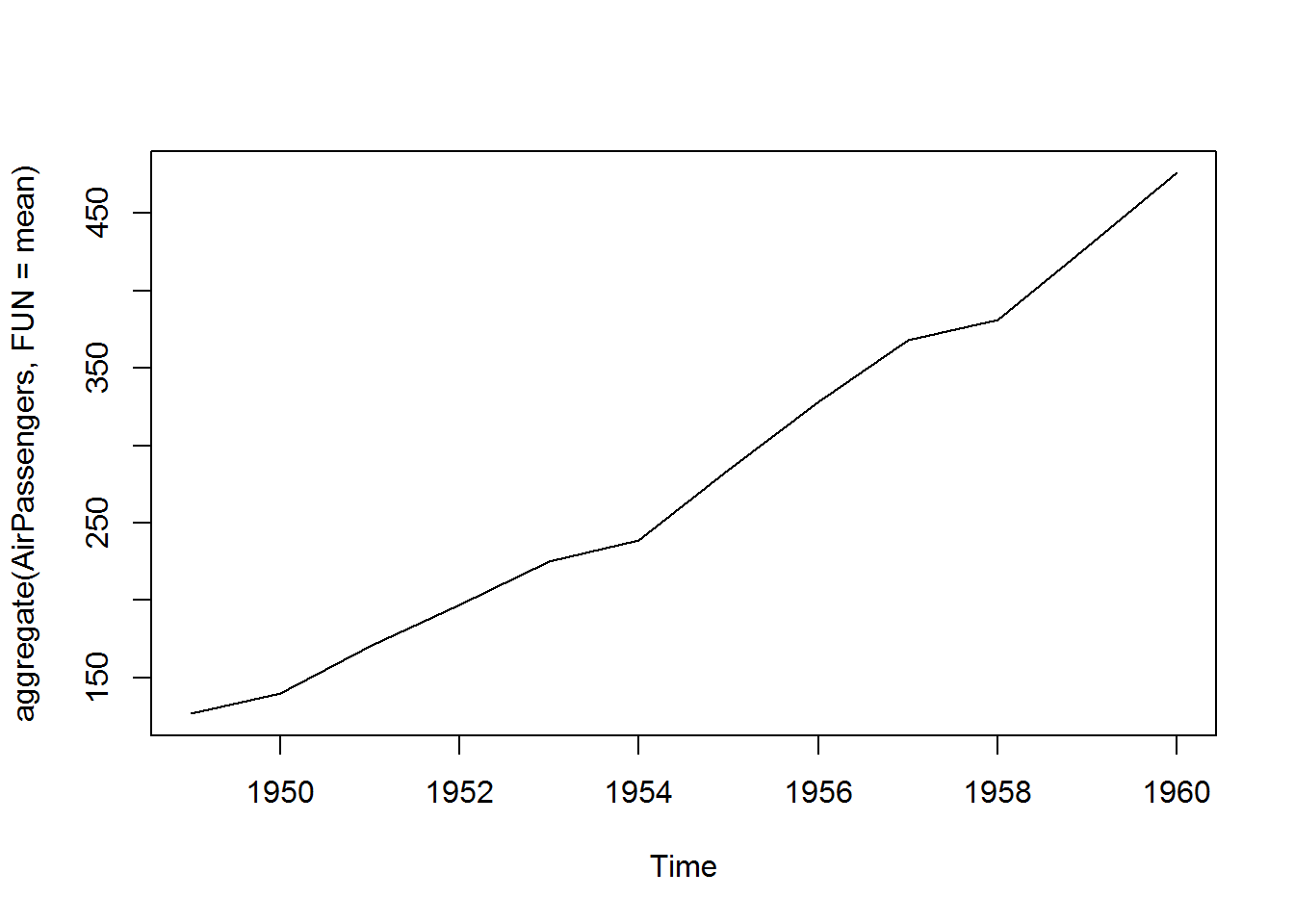
## boxplot on seasonal data
boxplot(AirPassengers~cycle(AirPassengers))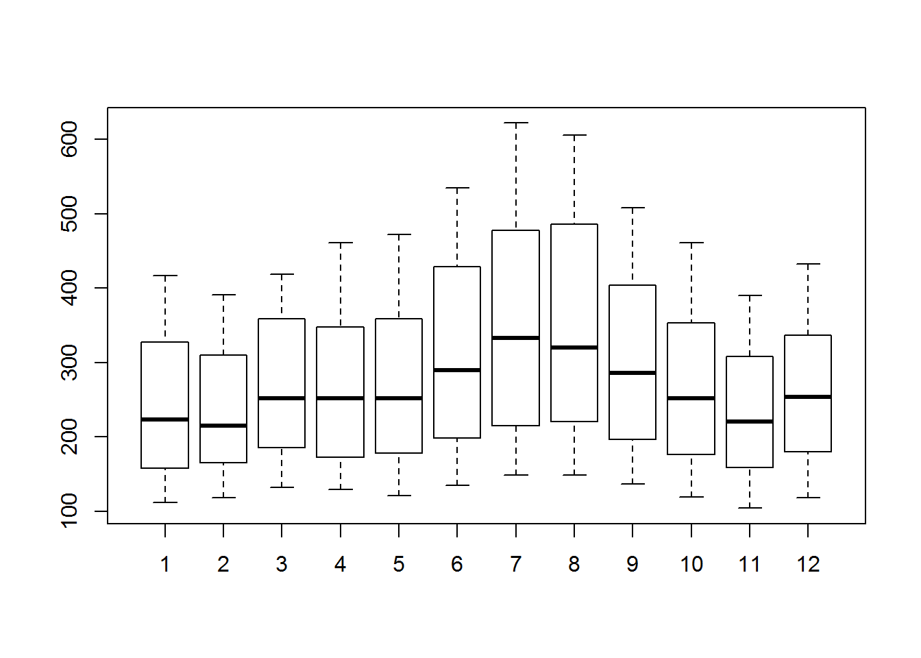
## The variance and the mean value in July and August is much higher than rest of the months.
## Even though the mean value of each month is quite different their variance is small.
## Hence, we have strong seasonal effect with a cycle of 12 months or less.
stationization
## remove unequal variance and address trend component
library(tseries)
adf.test(diff(log(AirPassengers)), alternative = "stationary", k = 0)
## Warning in adf.test(diff(log(AirPassengers)), alternative = "stationary", :
## p-value smaller than printed p-value##
## Augmented Dickey-Fuller Test
##
## data: diff(log(AirPassengers))
## Dickey-Fuller = -9.6003, Lag order = 0, p-value = 0.01
## alternative hypothesis: stationary# find parms for ARIMA model
## The ACF chart decays very slow, meaning the data is not stationary
acf(log(AirPassengers))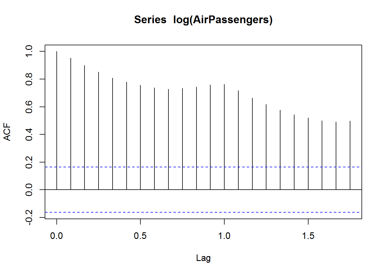
# Try diff
acf(diff(log(AirPassengers)))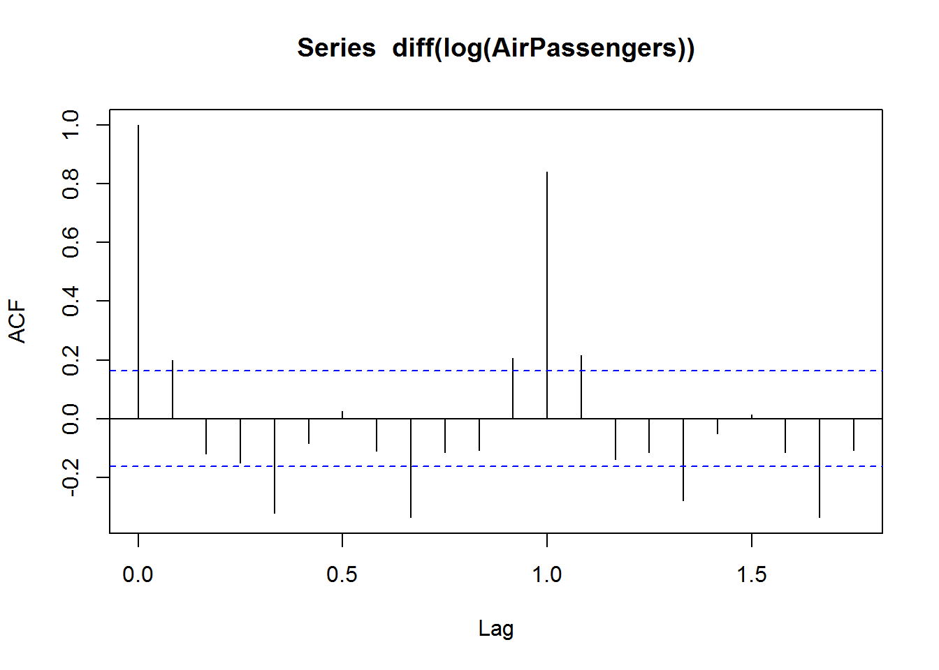
pacf(diff(log(AirPassengers)))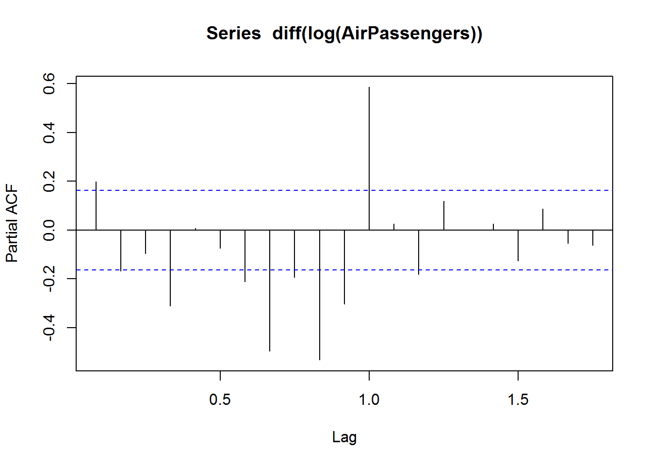
# get param (p,d,q) values
## The value of p should be 0 as the ACF is the curve getting a cut off
## choose (p,d,q) that have both lowest AIC, BIC
p <- 0
d <- 1
min_sum <- 0
final_q <- 1
for (q in c(1,2)) {
  fit <- arima(log(AirPassengers), c(p,d,q), seasonal = list(order = c(p,d,q), period = 12))
  sum <- AIC(fit) + BIC(fit)
  if (sum < min_sum) {
    min_sum <- sum
    final_q <- q
  }
}

final_q
## [1] 1# make prediction, 2.718 is e
fit <- arima(log(AirPassengers), c(p,d,final_q), seasonal = list(order = c(p,d,final_q), period = 12))
pred <- predict(fit, n.ahead = 6*12)
ts.plot(AirPassengers, 2.718^pred$pred, log = "y", lty = c(1,3))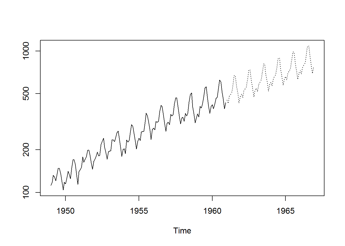

Share this post
Twitter
Google+
Facebook
Reddit
LinkedIn
StumbleUpon
Email